This tutorial provides a comprehensive guide to using PEtab-GUI for creating and managing PEtab parameter estimation problems for systems biology models.
PEtab-GUI is a graphical user interface for the PEtab format, which is a standardized way to specify parameter estimation problems in systems biology. This tutorial will guide you through the entire workflow of creating a parameter estimation problem using PEtab-GUI.
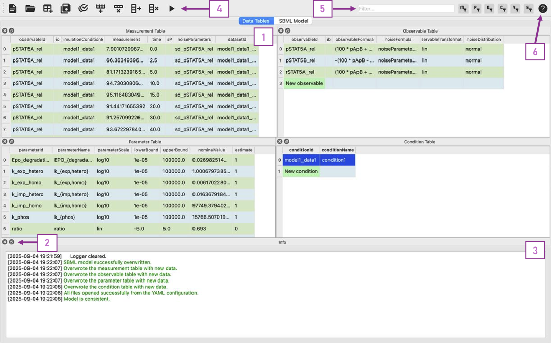
When you first launch PEtab-GUI, you’ll see the main window as shown below:
PEtab-GUI Main Window: (1) Every Table is in its own dockable panel. Using the buttons in (2) you can get each widget as a separate window or close it entirely. To reopen it, use the View menu in the menu bar.
(3) The Info widget shows log messages and clickable documentation links. Here you will be informed about deleted lines, potential validation problems and more. (4) The toolbar provides quick access to common actions
like opening/saving files, table modification, and model simulation. (5) The filter allows you to only look at specific rows. The filter buttons to the right let you select in which tables the filter should be applied.
(6) If you are unsure what to do, you can enter the Tutorial Mode by clicking the question mark icon in the toolbar. This will allow you to click different widgets or columns in the tables to get more information about their purpose.
The interface is organized into several key areas:
Menu Bar:
At the top, providing access to File, Edit, View, and Help. These items allow you to edit your PEtab problem and navigate the application. Most notably, the View menu allows you to toggle the visibility of the different panels.
Toolbar:
Below the menu bar, offering quick access to common actions like opening/saving files, table modification, and model simulation.
Main Window:
The main window of the application can be categorized into two main sections that can be selected via tab navigation:
Data Tables (left tab):
Six dockable table panels, each corresponding to a PEtab table (see also the PEtab Documentation):
Info panel: Displays log messages and clickable documentation links
Measurement Plot panel:
At the bottom, visualizes the measurement data based on your current model.
→ See: Validation and Inspection
SBML Model (right tab):
A built-in editor for creating and editing SBML models. It is split into two synced editors:
SBML Model Editor: For editing the SBML model directly.
Antimony Editor: For editing the Antimony representation of the model.
Changes in these can be forwarded to the other editor, allowing you to work in your preferred format.
→ See: Creating/Editing an SBML Model
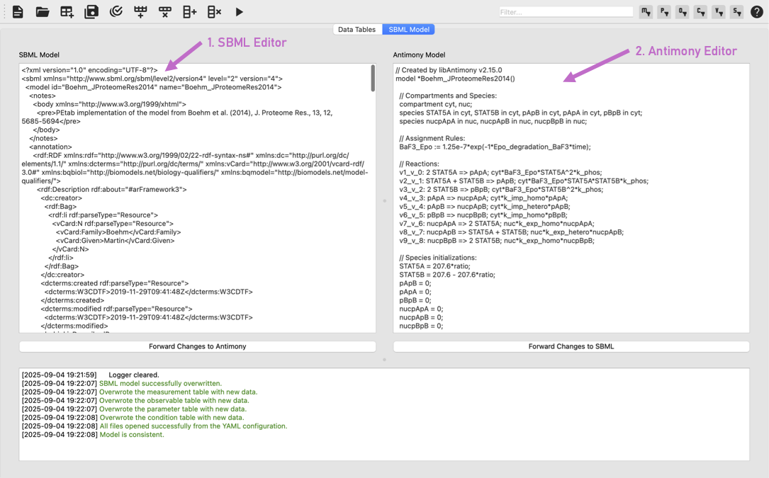
SBML and Antimony Editors: The second tab of the GUI application. The SBML editor (1) allows you to edit the SBML model directly, while the Antimony editor (2) provides a more human-readable format. Changes in one editor can be forwarded to the other using the buttons below them.
We can can now start creating a new PEtab problem or edit an existing one. The following sections will guide you through the process of defining and editing your model, experimental conditions, measurements, observables, and parameters.
While at each step we will learn about the different panels and how to fill the corresponding tables, it might be helpful to have a look at the PEtab Documentation (tutorial) to get a better understanding of the PEtab format and its requirements.
This section provides a complete, hands-on walkthrough to create your first PEtab parameter estimation problem from scratch.
You will create a simple conversion model where species A converts to species B, import measurement data for both species in matrix format, and validate the complete problem.
You can also watch a tutorial video covering similar steps and create your first PEtab problem alongside it.
What we’ll build: A model describing first-order conversion of species A to species B, with experimental measurements for both species at different time points.
Note
Expected time: 10-15 minutes
Sample data files: Download the example files from the GitHub repository
or create them as described below.
We’ll create a simple model using the Antimony editor.
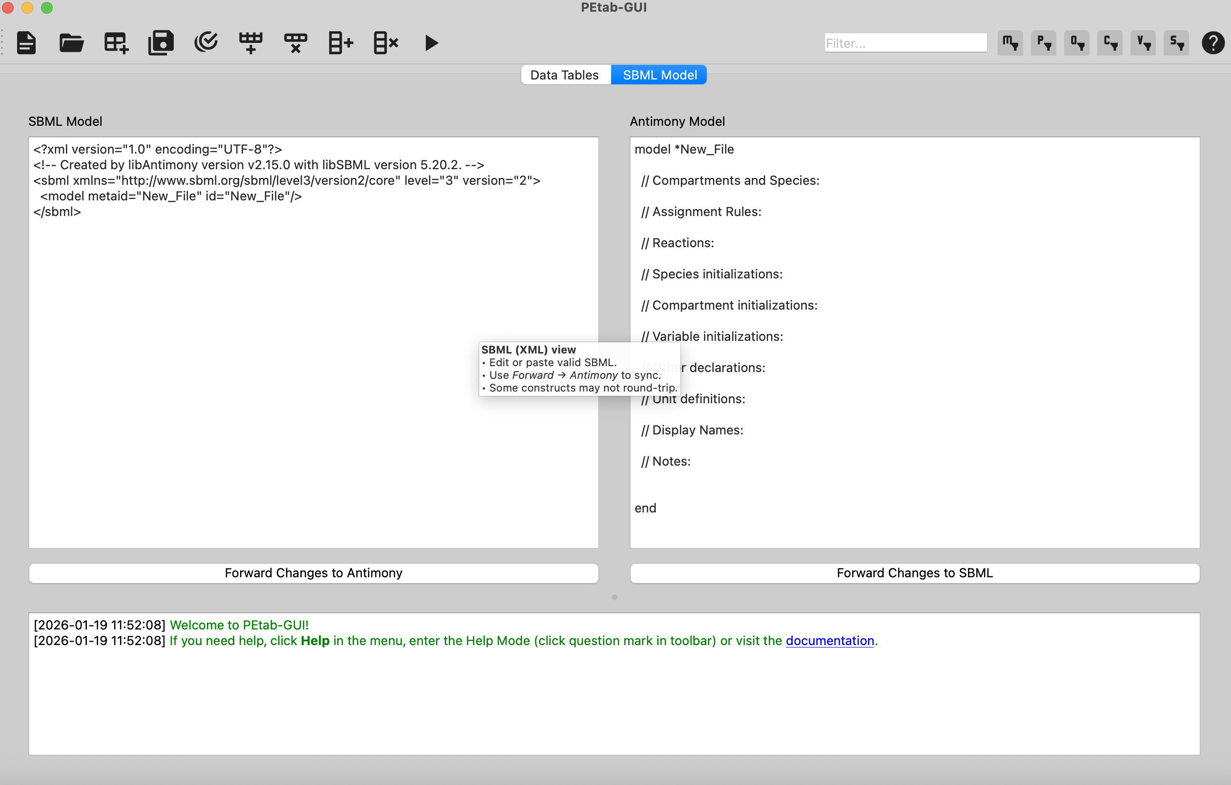
Click on the SBML Model tab at the top of the main window
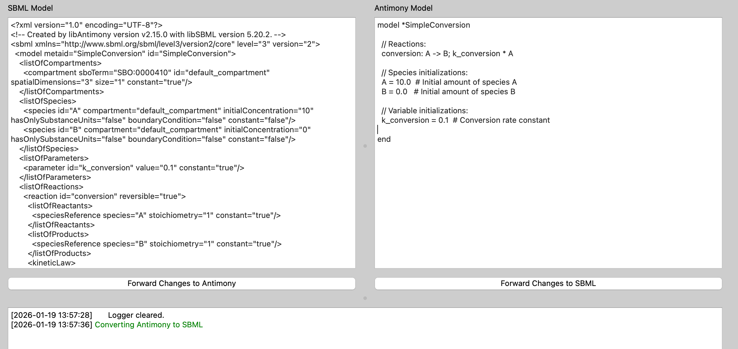
In the Antimony Editor panel (on the right), enter the following model:
model*SimpleConversion//Reactions:conversion:A->B;k_conversion*A//Speciesinitializations:A=10.0# Initial amount of species AB=0.0# Initial amount of species B//Variableinitializations:k_conversion=0.1# Conversion rate constantend
Click the “Forward changes to SBML” button below the Antimony editor
You should see the SBML XML representation appear in the SBML Model Editor (left panel)
Creating a simple conversion model in Antimony (right panel) and converting it to SBML (left panel).
What you should see: The SBML editor should now contain XML code with <listOfSpecies>, <listOfParameters> and <listOfReactions> elements.
The Info panel at the bottom might show a message confirming the conversion.
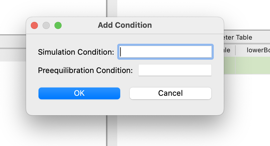
Then drag and drop this file onto the Measurement Table panel. When prompted, enter cond_1 for Simulation Condition.
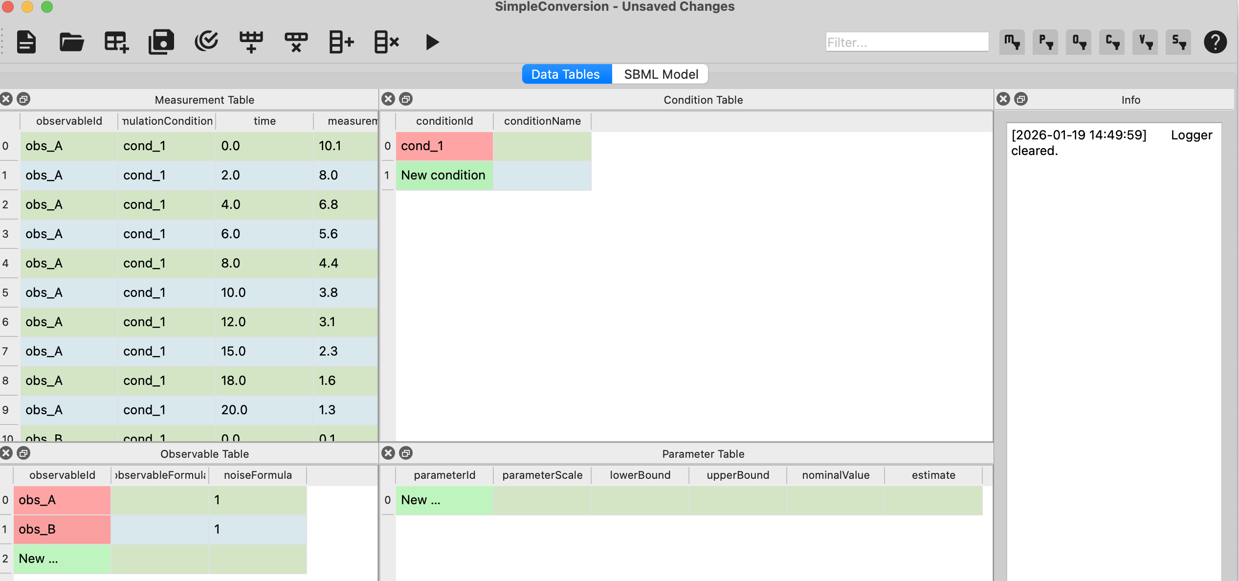
You should now see the measurements imported, the condition and observables created, but some things are marked red.
This is the petab linter telling you that some required fields are missing, namely the observable formula, which the GUI
can not set automatically. We will fix this in the next steps.
Dialog when uploading data matrix asking for SimulationConditionId.
What you should see: The Measurement Table should now contain 20 rows with your measurement data (10 time points for each of the two species).
The Info panel will likely show messages about auto-generated observables and conditions.
Measurement Table after importing data - 10 time points with measurements for both species A and B.
PEtab-GUI has automatically created observable entries for both species (obs_A and obs_B) in the Observable Table,
but we need to specify how these observables relate to our model species.
Locate the Observable Table panel (you may need to scroll or rearrange panels)
Find the row with observableId = obs_species_A
Click on the observableFormula cell (should be empty or have a placeholder)
Enter: A
This tells PEtab that the observable directly corresponds to the species A in our model.
In the noiseFormula cell, enter: 0.5
This specifies that measurements have a standard deviation of 0.5 units (normally distributed noise).
Now find the row with observableId = obs_species_B
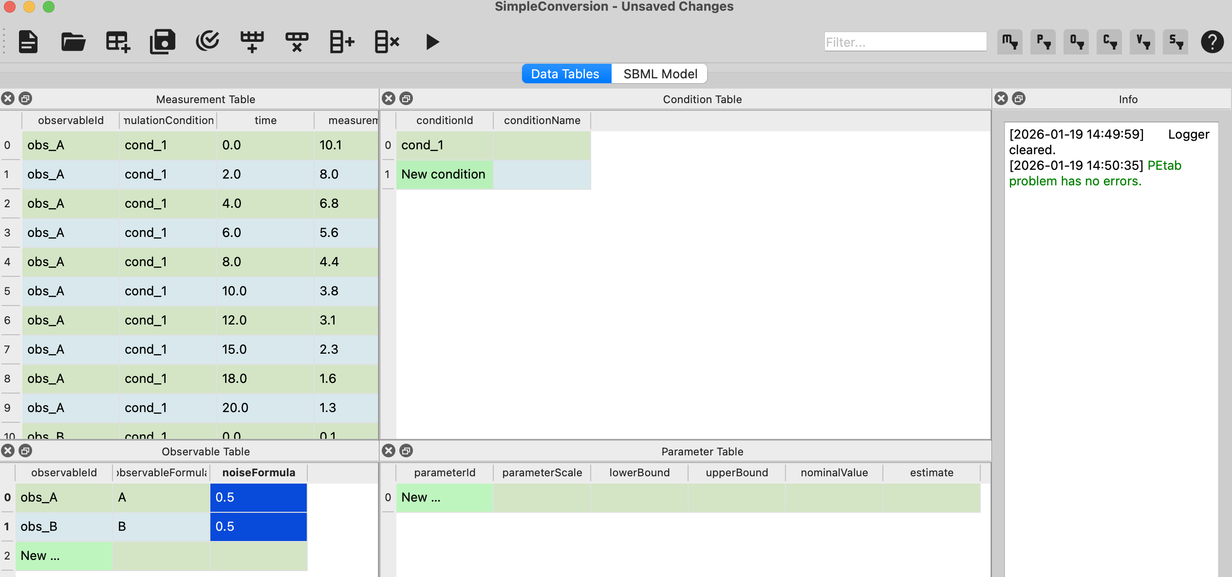
In the observableFormula cell, enter: B
In the noiseFormula cell, enter: 0.5
Click Check PEtab in the Toolbar.
You should now see a complete observable table and no more errors in the Info panel.
Observable Table with formulas for both species A and B, each with noise standard deviation set to 0.5.
What you should see: The Info panel might show validation messages confirming the observables are now properly defined.
What you should see: PEtab-GUI has automatically created an entry for cond_1 (referenced in your measurements).
Since our simple model doesn’t require any condition-specific parameter overrides or initial value changes, this table
can remain as-is with just the conditionId column filled. If you want to rename it, just edit the cell in the
Condition Table and when subsequently approved, the condition IDs in the Measurement Table will be updated accordingly.
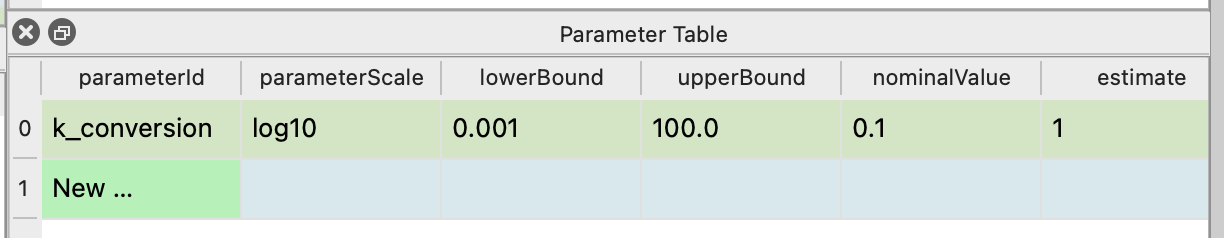
Now we specify which parameters should be estimated and their bounds.
Switch to the Parameter Table panel
Click the “Add Row” button in the toolbar (or use Edit ‣ Add Row) or just add it directly
by double clicking in the first empty row.
Start filling in k_, you should automatically be prompted to select k_conversion from a dropdown of model parameters.
The nominalValue will be taken from your SBML model, the parameterScale should be set to log10 by default and estimate should set to 1.
You only need to fill out the lower and upper bounds now. Fill in 0.001 and 100 respectively.
Note
We use log10 scale because rate constants often span several orders of magnitude, and optimization works better in log space.
Feel free to use linear scale for parameters as you see fit.
Parameter Table configured for estimating k_conversion with bounds [0.001, 100] on log10 scale.
What you should see: One row in the Parameter Table with all columns filled. Nothing should be colored red anymore.
Make sure the Data Plot panel is visible at the bottom
(if not, enable it via View ‣ Data Plot)
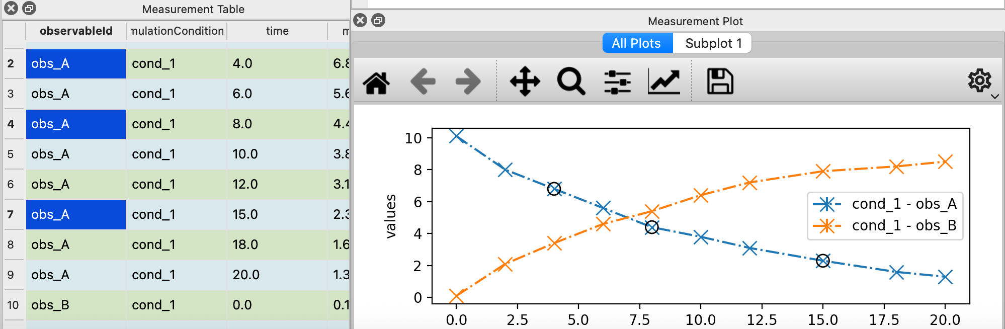
You should see two plot with time on the x-axis and measurement values on the y-axis, one for obs_A and one for obs_B.
If you want to see only one plot with both species, click the cogwheel icon in the Measurement Plot panel and select Group by condition.
The plot should show two sets of data points: one for species A (decreasing over time) and one for species B (increasing over time), with about 10 time points each.
Measurement Plot showing the experimental data - time points vs. measured values for both species A (decreasing) and species B (increasing).
Try this: In the Measurement Table select one or multiple rows. The corresponding point(s) in the
Data Plot will be highlighted. This linking lets you explore and validate your data early on.
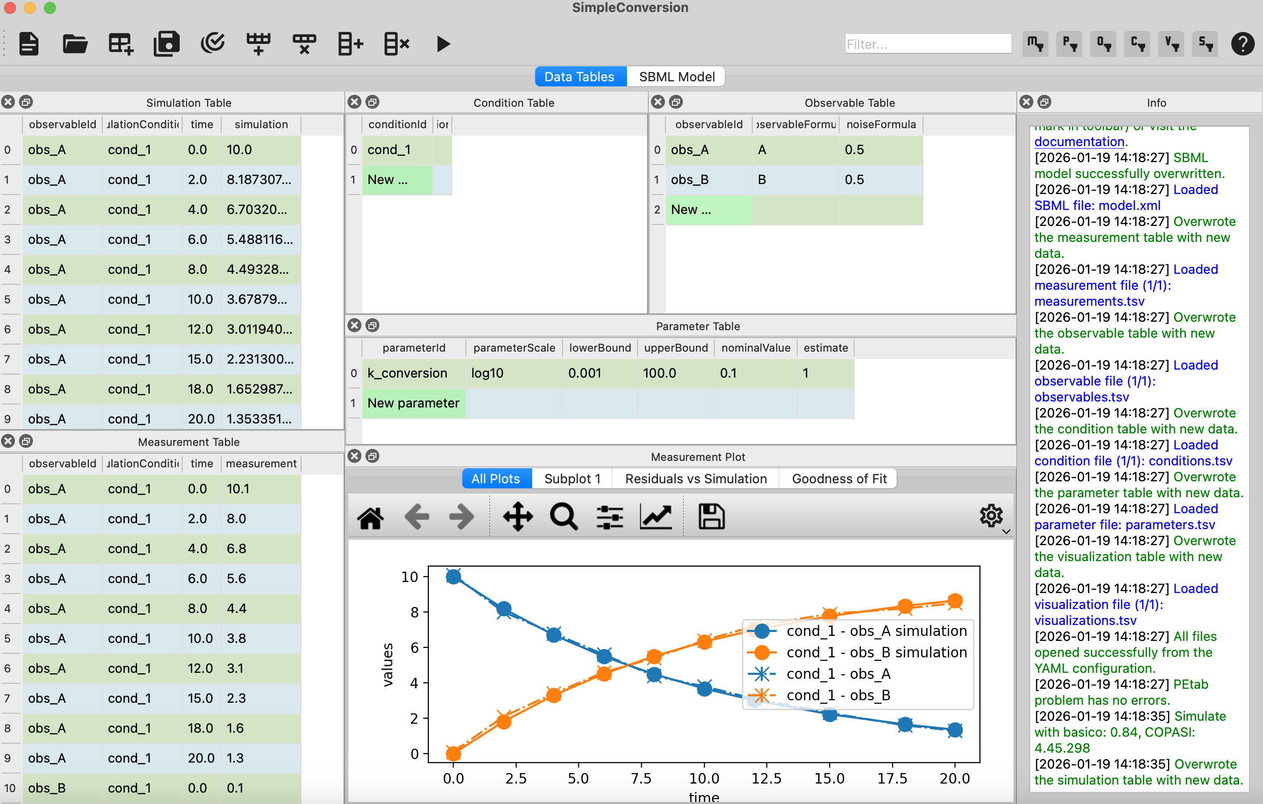
Now let’s simulate the model with our current parameter values to see how well it fits the data.
In the toolbar, click the “Simulate” button (usually has a “play” or “gear” icon)
Wait a few seconds for the simulation to complete
The Simulation Table panel should appear (if not, enable it via View ‣ Simulation Table)
In the Data Plot panel - you should now see both your measurements (dots) and the simulation (lines)
Measurement Plot after running simulation - measurements (dots) and model simulation (lines) are shown together for both species A and B. The conversion rate k_conversion=0.1 provides a good fit to the data.
What you should see: Two line plots overlaid on your measurement points - one for species A (decreasing) and one for species B (increasing). If you used the exact values from this tutorial,
the simulation should match the measurements reasonably well since the data was generated with k_conversion ≈ 0.1.
If you already have a PEtab problem defined in a YAML file or you have your SBML model already, you can open them directly in PEtab-GUI:
Through the menu bar, go to File ‣ Open. This will open a file dialog, where you can select your YAML file, SBML model file, or any other PEtab-related files.
Alternatively, you can drag and drop your YAML file onto the PEtab-GUI window. The application will automatically handle the file and load the relevant data into the interface.
If you want to continue working on an existing PEtab problem, you can also use the File ‣ Recent Files menu to quickly access recently opened projects.
Since a PEtab problem consists of several components, we will go through the process step by step. The following sections will guide you through creating or editing a PEtab problem using the PEtab-GUI.
While there is no strict order in which you have to fill the tables, we will follow a logical sequence that starts with the model definition, followed by measurements, experimental conditions, observables, and parameters.
Usually the first step in creating a PEtab problem is to define the underlying SBML model.
Independent of whether you are creating a new model or editing an existing one, you are given the choice between editing
the model directly in SBML or in the much more readable
Antimony and then converting it to SBML.
💡 Need help understanding what an SBML model is?
SBML (Systems Biology Markup Language) is an XML-based format for representing computational models of biological processes.
It describes the components of a biological system:
Species: Molecular entities (proteins, metabolites, genes, etc.) that can change over time
Reactions: Processes that transform species (e.g., enzymatic reactions, binding/unbinding events)
Parameters: Constants that define reaction rates, initial concentrations, and other quantities
Compartments: Physical locations where species exist (e.g., cytoplasm, nucleus, extracellular space)
SBML files are typically generated by modeling tools or written programmatically. While SBML is precise and machine-readable,
it can be verbose and difficult to read/write manually. That’s why PEtab-GUI supports Antimony, a human-readable text
format that can be easily converted to SBML. If you’re new to biological modeling, we recommend starting with Antimony
and converting to SBML when needed.
If you are creating a new model, the empty antimony template might help in getting started.
Here is a simple example showcasing how species, reactions, and parameters can be defined:
model*ExampleModel//ReactionsJ0:S1->S2+S3;k1*S1# Mass-action kineticsJ1:S2->S3+S4;k2*S2//SpeciesinitializationS1=10# The initial concentration of S1S2=0# The initial concentration of S3S3=3# The initial concentration of S3S4=0# The initial concentration of S4//Variableinitializationk1=0.1# The value of the kinetic parameter from J0.k2=0.2# The value of the kinetic parameter from J1.end
Indispensable for parameter estimation problems are the measurements that will be used to fit the model parameters.
In PEtab-GUI, you can define these measurements in the Measurement Table.
While it is possible to create a new measurement table from scratch, it is usually more convenient to import an already
existing measurement file. In our experience, most measurements exist in some matrix format. Time-resolved data might have each
row corresponding to a time point and each column corresponding to a different observable.
Similar can Dose-Response data be structured, where each row corresponds to a different dose.
Accounting for these common formats, PEtab-GUI handles opening a CSV or TSV file by checking whether it is a time series,
dose-response, or a PEtab measurement file. Simply drag and drop your file into the Measurement Table or
use the File ‣ Open option. In general what we need to specify in the measurement table are:
observableId: A unique identifier for the observable that this measurement corresponds to. This should match the observable IDs defined in the Observable Table.
simulationConditionId: The condition under which the measurement was taken. You are free to choose a name but it should be consistent with the conditions defined in the Condition Table.
time and measurement: The time point and corresponding measurements.
There are a number of optional columns that can be specified, for more details see the PEtab Documentation.
One of PEtab-GUI’s most powerful features is its ability to automatically convert matrix-format experimental data into PEtab format.
This is particularly useful because most experimental data is initially organized in matrix layouts.
Common matrix formats:
Time-series data: Rows = time points, Columns = different conditions or replicates
Dose-response data: Rows = different doses, Columns = different observables or replicates
Multi-condition experiments: Any tabular layout where measurements are organized by experimental variables
First column (time): The independent variable (time, dose, etc.)
Other columns: Measurement values for different conditions
Column headers: Become condition names or observable names
This needs to be converted to PEtab’s “long format” where each measurement is a separate row with explicit
observableId, simulationConditionId, time, and measurement columns.
Let’s walk through importing the matrix data shown above.
Step 1: Prepare Your Matrix File
Create a CSV or TSV file with your matrix data. Requirements:
First row must contain column headers
First column should be the independent variable (typically time or dose)
Remaining columns contain measurement values
Use clear, descriptive column names (they will become observable IDs)
Step 2: Import the Matrix File
Make sure you have an SBML model already loaded (PEtab-GUI needs to know what species exist)
In the Data Tables tab, locate the Measurement Table panel
Drag and drop your file onto the Measurement Table
OR
Use File ‣ Open and select your matrix file
When prompted, enter the name for the simulationConditionId column (e.g., condition)
Step 3: Watch the Automatic Conversion
PEtab-GUI will automatically:
Detect that your file is in matrix format (not already in PEtab format)
Convert the matrix to PEtab long format:
Each cell in the matrix becomes a separate row in the Measurement Table
Column names become simulationConditionId values (control, low_dose, etc.)
The first column values become time values
Cell values become measurement values
Generate observables: Create entries in the Observable Table (one per matrix column)
Generate conditions: Create entries in the Condition Table (as per Prompt)
Step 4: Complete the Observable Definitions
The auto-generated observables need their formulas defined:
Switch to the Observable Table
For each observable (e.g., obs_A, obs_B), fill in the observableFormula column
Fill in the noiseFormula column (e.g., 0.5 for constant noise, or 0.1*A for proportional noise)
Example Observable Table after completion:
observableId | observableFormula | noiseFormula
obs_A        | A                 | 0.5
obs_A        | A                 | 0.5
obs_A        | A                 | 0.5
obs_B        | B                 | 0.5
Step 5: Verify and Visualize
Run a lint check to verify everything is correctly configured
View the Measurement Plot to see all your data visualized
Run a simulation to see how your model fits the data
Observables define how model species are mapped to measured quantities. When you create a measurement in the
Measurement Table, you need to specify which observable it corresponds to. If it is not already defined, PEtab-GUI
will automatically create a new observable entry in the Observable Table. You will only have to fill out the actual
function in the observableFormula column, which defines how the observable is calculated from the model species. In
the easiest case, this just corresponds to the species ID, e.g. S1. But it could also be a more complex expression like
k_scale*(S1+S2), that even introduces new parameters, e.g. k_scale.
In general, we assume that the measurement is subject to some noise. Per default the noise is normally distributed and
within the noiseFormula column you can specify the standard deviation of the noise. Again, this formula can be a
simple number or a more complex formula introducing new parameters.
For more details, for example on how to change the noise model, see the PEtab Documentation.
Experimental conditions define the specific settings under which measurements were taken. Aside from the conditionId column,
all other columns are optional. The other columns may either set a parameter to take different values across the conditions
or an initial value for a species that is different across conditions (e.g. in case of a dose-response experiment).
Just as in the observable table, new conditions can be created automatically when you create a new measurement in the Measurement Table.
The last thing you will want to fill out is the Parameter Table. This table defines the parameters that
are part of the estimation problem. This includes parameters from the SBML model, observables, and noise models.
For every parameter you declare in the estimate column whether it should be estimated during the parameter estimation or not.
Additionally you specify lower and upper bounds for the parameter values in the lowerBound and upperBound columns, respectively.
If your parameter is not to be estimated, you need to specify a nominalValue. PEtab-GUI aids you in this process by suggesting
parameter IDs from the SBML model you might want to add here.
Once you have filled out all the tables, it is important to validate your PEtab problem to avoid errors during parameter estimation.
PEtab-GUI supports this through Visualization and Simulation and Linting features:
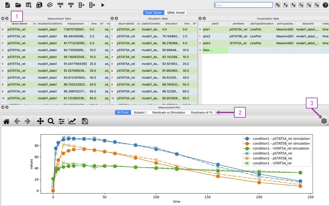
PEtab-GUI with Visualization and Simulation Panels: Once you have defined measurements, you can add the Measurement Plot to visualize your measurements. You can also add the Simulation Table and Visualization Table to run simulations and visualize the results.
(1) The three tables can be neatly arranged next to each other. (2) Within the measurement panel, you can click on different plots. If you have specified multiple plots, All Plots will show every plot specified, followed by tabs for each individual plot.
If you have simulations you additionally get a residual plot and a scatterplot of the fit. Through the settings symbol (3) you can change whether you want to plot by observable, condition or defined by the visualization table.
In the Measurement Plot panel, you will see a visualization of your measurements. You can click on individual points in the
measurement plot to see the corresponding measurement in the Measurement Table and vice versa. This can already help getting an
idea of the dynamics of your model and spot potential outliers in your measurements.
Once you have defined all the necessary components, you might want to see whether a specific parameter set leads to a good fit of the model to the measurements.
For this you can add two panels to the main interface, the Simulation Table and the Visualization Table.
The Simulation Table panel is strictly speaking not part of the PEtab problem definition.
Structurally it is the same as the Measurement Plot panel, with the sole difference that the column measurement
is replaced by simulation.
The Visualization Table allows you to specify how the measurements (and simulations) should be visualized. In short:
every plotId corresponds to a specific plot. Rows that have the same plotId will be plotted together.
You specify your xValues and yValues for each row.
You can specify additional details, such as offsets and scale. For more details see the PEtab Documentation.
If you dont have simulations yet, you can run a Simulation through the toolbar button, which will automatically fill the Simulation Table,
running a simulation with the current parameter values and conditions.
If you have simulations, additional plots can be viewed, such as residual plots, as well as goodness-of-fit plots.
Linting is the process of automatically checking your tables for structural and logical errors during editing.
PEtab-GUI offers two layers of linting support:
Partial Linting on Edit:
Whenever you modify a single row in any table, PEtab-GUI will immediately lint that row in context.
This allows you to catch errors as you build your PEtab problem — such as missing required fields, mismatched IDs, invalid references, or inconsistent units.
Full Model Linting:
You can run a complete validation of your PEtab problem by clicking the lint icon in the toolbar.
This performs a full consistency check across all tables and provides more comprehensive diagnostics.
All linting messages — including errors and warnings — appear in the Info panel at the bottom right of the interface.
Messages include timestamps, color coding (e.g., red for errors, orange for warnings), and sometimes clickable references or hints.
By using linting early and often, you can avoid many common errors in PEtab problem definition and ensure compatibility with downstream tools.
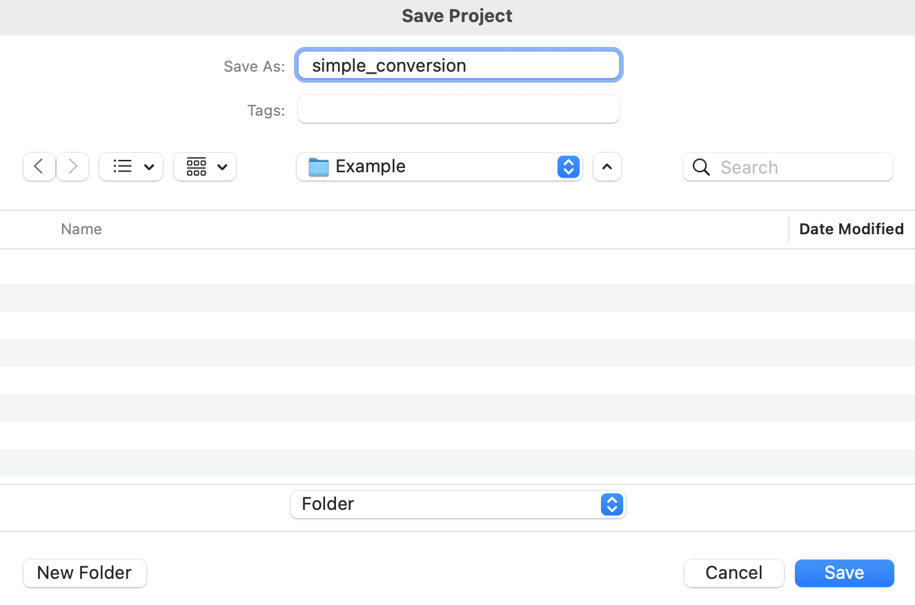
Once you’ve set up your parameter estimation problem, and sufficiently validated it, you can save your project. This
can be done either as a compressed ZIP file or as a COMBINE archive.
You can also save each table as a separate CSV file.